Basic Principles of Spark
Note
The Spark component applies to versions earlier than MRS 3.x.
Description
Spark is an open source parallel data processing framework. It helps you easily develop unified big data applications and perform offline processing, stream processing, and interactive analysis on data.
Spark provides a framework featuring fast computing, write, and interactive query. Spark has obvious advantages over Hadoop in terms of performance. Spark uses the in-memory computing mode to avoid I/O bottlenecks in scenarios where multiple tasks in a MapReduce workflow process the same dataset. Spark is implemented by using Scala programming language. Scala enables distributed datasets to be processed in a method that is the same as that of processing local data. In addition to interactive data analysis, Spark supports interactive data mining. Spark adopts in-memory computing, which facilitates iterative computing. By coincidence, iterative computing of the same data is a general problem facing data mining. In addition, Spark can run in Yarn clusters where Hadoop 2.0 is installed. The reason why Spark cannot only retain various features like MapReduce fault tolerance, data localization, and scalability but also ensure high performance and avoid busy disk I/Os is that a memory abstraction structure called Resilient Distributed Dataset (RDD) is created for Spark.
Original distributed memory abstraction, for example, key-value store and databases, supports small-granularity update of variable status. This requires backup of data or log updates to ensure fault tolerance. Consequently, a large amount of I/O consumption is brought about to data-intensive workflows. For the RDD, it has only one set of restricted APIs and only supports large-granularity update, for example, map and join. In this way, Spark only needs to record the transformation operation logs generated during data establishment to ensure fault tolerance without recording a complete dataset. This data transformation link record is a source for tracing a data set. Generally, parallel applications apply the same computing process for a large dataset. Therefore, the limit to the mentioned large-granularity update is not large. As described in Spark theses, the RDD can function as multiple different computing frameworks, for example, programming models of MapReduce and Pregel. In addition, Spark allows you to explicitly make a data transformation process be persistent on hard disks. Data localization is implemented by allowing you to control data partitions based on the key value of each record. (An obvious advantage of this method is that two copies of data to be associated will be hashed in the same mode.) If memory usage exceeds the physical limit, Spark writes relatively large partitions into hard disks, thereby ensuring scalability.
Spark has the following features:
Fast: The data processing speed of Spark is 10 to 100 times higher than that of MapReduce.
Easy-to-use: Java, Scala, and Python can be used to simply and quickly compile parallel applications for processing massive amounts of data. Spark provides over 80 operators to help you compile parallel applications.
Universal: Spark provides many tools, for example, Spark SQL and Spark Streaming. These tools can be combined flexibly in an application.
Integration with Hadoop: Spark can directly run in a Hadoop cluster and read existing Hadoop data.
The Spark component of MRS has the following advantages:
The Spark Streaming component of MRS supports real-time data processing rather than triggering as scheduled.
The Spark component of MRS provides Structured Streaming and allows you to build streaming applications using the Dataset API. Spark supports exactly-once semantics and inner and outer joins for streams.
The Spark component of MRS uses pandas_udf to replace the original user-defined functions (UDFs) in PySpark to process data, which reduces the processing duration by 60% to 90% (affected by specific operations).
The Spark component of MRS also supports graph data processing and allows modeling using graphs during graph computing.
Spark SQL of MRS is compatible with some Hive syntax (based on the 64 SQL statements of the Hive-Test-benchmark test set) and standard SQL syntax (based on the 99 SQL statements of the TPC-DS test set).
For details about Spark architecture and principles, visit https://archive.apache.org/dist/spark/docs/3.1.1/quick-start.html.
Architecture
Figure 1 describes the Spark architecture and Table 1 lists the Spark modules.
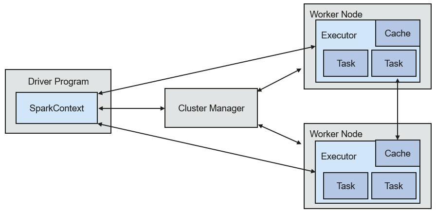
Figure 1 Spark architecture
Module | Description |
|---|---|
Cluster Manager | Cluster manager manages resources in the cluster. Spark supports multiple cluster managers, including Mesos, Yarn, and the Standalone cluster manager that is delivered with Spark. |
Application | Spark application. It consists of one Driver Program and multiple executors. |
Deploy Mode | Deployment in cluster or client mode. In cluster mode, the driver runs on a node inside the cluster. In client mode, the driver runs on the client (outside the cluster). |
Driver Program | The main process of the Spark application. It runs the main() function of an application and creates SparkContext. It is used for parsing applications, generating stages, and scheduling tasks to executors. Usually, SparkContext represents Driver Program. |
Executor | A process started on a Work Node. It is used to execute tasks, and manage and process the data used in applications. A Spark application usually contains multiple executors. Each executor receives commands from the driver and executes one or multiple tasks. |
Worker Node | A node that starts and manages executors and resources in a cluster. |
Job | A job consists of multiple concurrent tasks. One action operator (for example, a collect operator) maps to one job. |
Stage | Each job consists of multiple stages. Each stage is a task set, which is separated by Directed Acyclic Graph (DAG). |
Task | A task carries the computation unit of the service logics. It is the minimum working unit that can be executed on the Spark platform. An application can be divided into multiple tasks based on the execution plan and computation amount. |
Spark Application Running Principle
Figure 2 shows the Spark application running architecture. The running process is as follows:
An application is running in the cluster as a collection of processes. Driver coordinates the running of the application.
To run an application, Driver connects to the cluster manager (such as Standalone, Mesos, and Yarn) to apply for the executor resources, and start ExecutorBackend. The cluster manager schedules resources between different applications. Driver schedules DAGs, divides stages, and generates tasks for the application at the same time.
Then, Spark sends the codes of the application (the codes transferred to SparkContext, which is defined by JAR or Python) to an executor.
After all tasks are finished, the running of the user application is stopped.
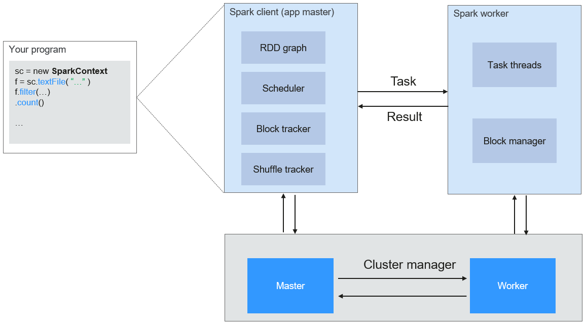
Figure 2 Spark application running architecture
Figure 3 shows the Master and Worker modes adopted by Spark. A user submits an application on the Spark client, and then the scheduler divides a job into multiple tasks and sends the tasks to each Worker for execution. Each Worker reports the computation results to Driver (Master), and then the Driver aggregates and returns the results to the client.
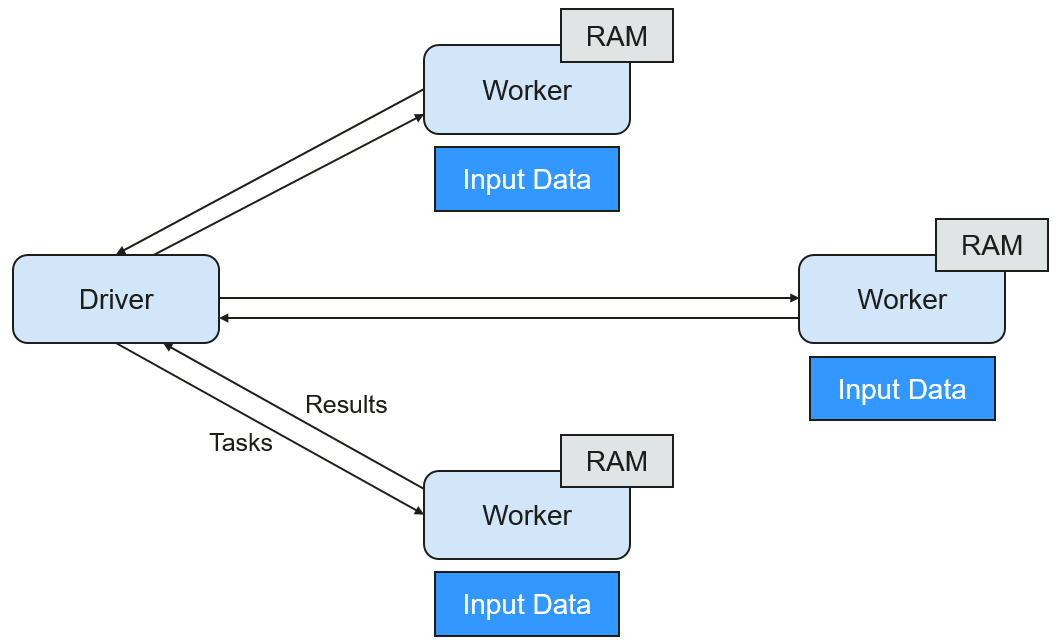
Figure 3 Spark Master-Worker mode
Note the following about the architecture:
Applications are isolated from each other.
Each application has an independent executor process, and each executor starts multiple threads to execute tasks in parallel. Whether in terms of scheduling or task running on executors. Each driver independently schedules its own tasks. Different application tasks run on different JVMs, that is, different executors.
Different Spark applications do not share data, unless data is stored in the external storage system such as HDFS.
You are advised to deploy the Driver program in a location that is close to the Worker node because the Driver program schedules tasks in the cluster. For example, deploy the Driver program on the network where the Worker node is located.
Spark on YARN can be deployed in two modes:
In Yarn-cluster mode, the Spark driver runs inside an ApplicationMaster process which is managed by Yarn in the cluster. After the ApplicationMaster is started, the client can exit without interrupting service running.
In Yarn-client mode, the driver is started in the client process, and the ApplicationMaster process is used only to apply for resources from the Yarn cluster.
Spark Streaming Principle
Spark Streaming is a real-time computing framework built on the Spark, which expands the capability for processing massive streaming data. Currently, Spark supports the following data processing methods:
Direct Streaming
In Direct Streaming approach, Direct API is used to process data. Take Kafka Direct API as an example. Direct API provides offset location that each batch range will read from, which is much simpler than starting a receiver to continuously receive data from Kafka and written data to write-ahead logs (WALs). Then, each batch job is running and the corresponding offset data is ready in Kafka. These offset information can be securely stored in the checkpoint file and read by applications that failed to start.
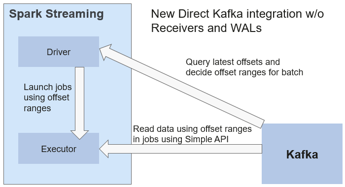
Figure 4 Data transmission through Direct Kafka API
After the failure, Spark Streaming can read data from Kafka again and process the data segment. The processing result is the same no matter Spark Streaming fails or not, because the semantic is processed only once.
Direct API does not need to use the WAL and Receivers, and ensures that each Kafka record is received only once, which is more efficient. In this way, the Spark Streaming and Kafka can be well integrated, making streaming channels be featured with high fault-tolerance, high efficiency, and ease-of-use. Therefore, you are advised to use Direct Streaming to process data.
Receiver
When a Spark Streaming application starts (that is, when the driver starts), the related StreamingContext (the basis of all streaming functions) uses SparkContext to start the receiver to become a long-term running task. These receivers receive and save streaming data to the Spark memory for processing. Figure 5 shows the data transfer lifecycle.
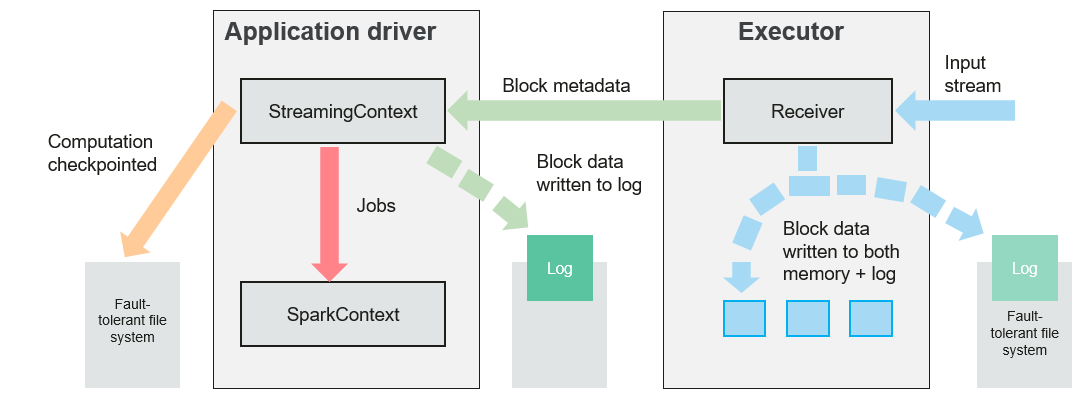
Figure 5 Data transfer lifecycle
Receive data (blue arrow).
Receiver divides a data stream into a series of blocks and stores them in the executor memory. In addition, after WAL is enabled, it writes data to the WAL of the fault-tolerant file system.
Notify the driver (green arrow).
The metadata in the received block is sent to StreamingContext in the driver. The metadata includes:
Block reference ID used to locate the data position in the Executor memory.
Block data offset information in logs (if the WAL function is enabled).
Process data (red arrow).
For each batch of data, StreamingContext uses block information to generate resilient distributed datasets (RDDs) and jobs. StreamingContext executes jobs by running tasks to process blocks in the executor memory.
Periodically set checkpoints (orange arrows).
For fault tolerance, StreamingContext periodically sets checkpoints and saves them to external file systems.
Fault Tolerance
Spark and its RDD allow seamless processing of failures of any Worker node in the cluster. Spark Streaming is built on top of Spark. Therefore, the Worker node of Spark Streaming also has the same fault tolerance capability. However, Spark Streaming needs to run properly in case of long-time running. Therefore, Spark must be able to recover from faults through the driver process (main process that coordinates all Workers). This poses challenges to the Spark driver fault-tolerance because the Spark driver may be any user application implemented in any computation mode. However, Spark Streaming has internal computation architecture. That is, it periodically executes the same Spark computation in each batch data. Such architecture allows it to periodically store checkpoints to reliable storage space and recover them upon the restart of Driver.
For source data such as files, the Driver recovery mechanism can ensure zero data loss because all data is stored in a fault-tolerant file system such as HDFS. However, for other data sources such as Kafka and Flume, some received data is cached only in memory and may be lost before being processed. This is caused by the distribution operation mode of Spark applications. When the driver process fails, all executors running in the Cluster Manager, together with all data in the memory, are terminated. To avoid such data loss, the WAL function is added to Spark Streaming.
WAL is often used in databases and file systems to ensure persistence of any data operation. That is, first record an operation to a persistent log and perform this operation on data. If the operation fails, the system is recovered by reading the log and re-applying the preset operation. The following describes how to use WAL to ensure persistence of received data:
Receiver is used to receive data from data sources such as Kafka. As a long-time running task in Executor, Receiver receives data, and also confirms received data if supported by data sources. Received data is stored in the Executor memory, and Driver delivers a task to Executor for processing.
After WAL is enabled, all received data is stored to log files in the fault-tolerant file system. Therefore, the received data does not lose even if Spark Streaming fails. Besides, receiver checks correctness of received data only after the data is pre-written into logs. Data that is cached but not stored can be sent again by data sources after the driver restarts. These two mechanisms ensure zero data loss. That is, all data is recovered from logs or re-sent by data sources.
To enable the WAL function, perform the following operations:
Set streamingContext.checkpoint to configure the checkpoint directory, which is an HDFS file path used to store streaming checkpoints and WALs.
Set spark.streaming.receiver.writeAheadLog.enable of SparkConf to true (the default value is false).
After WAL is enabled, all receivers have the advantage of recovering from reliable received data. You are advised to disable the multi-replica mechanism because the fault-tolerant file system of WAL may also replicate the data.
Note
The data receiving throughput is lowered after WAL is enabled. All data is written into the fault-tolerant file system. As a result, the write throughput of the file system and the network bandwidth for data replication may become the potential bottleneck. To solve this problem, you are advised to create more receivers to increase the degree of data receiving parallelism or use better hardware to improve the throughput of the fault-tolerant file system.
Recovery Process
When a failed driver is restarted, restart it as follows:
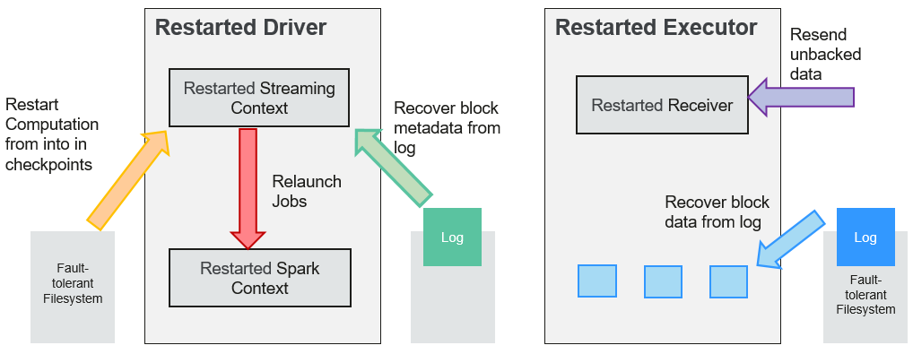
Figure 6 Computing recovery process
Recover computing. (Orange arrow)
Use checkpoint information to restart Driver, reconstruct SparkContext and restart Receiver.
Recover metadata block. (Green arrow)
This operation ensures that all necessary metadata blocks are recovered to continue the subsequent computing recovery.
Relaunch unfinished jobs. (Red arrow)
Recovered metadata is used to generate RDDs and corresponding jobs for interrupted batch processing due to failures.
Read block data saved in logs. (Blue arrow)
Block data is directly read from WALs during execution of the preceding jobs, and therefore all essential data reliably stored in logs is recovered.
Resend unconfirmed data. (Purple arrow)
Data that is cached but not stored to logs upon failures is re-sent by data sources, because the receiver does not confirm the data.
Therefore, by using WALs and reliable Receiver, Spark Streaming can avoid input data loss caused by Driver failures.
SparkSQL and DataSet Principle
SparkSQL
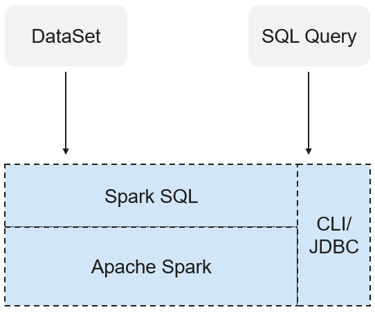
Figure 7 SparkSQL and DataSet
Spark SQL is a module for processing structured data. In Spark application, SQL statements or DataSet APIs can be seamlessly used for querying structured data.
Spark SQL and DataSet also provide a universal method for accessing multiple data sources such as Hive, CSV, Parquet, ORC, JSON, and JDBC. These data sources also allow data interaction. Spark SQL reuses the Hive frontend processing logic and metadata processing module. With the Spark SQL, you can directly query existing Hive data.
In addition, Spark SQL also provides API, CLI, and JDBC APIs, allowing diverse accesses to the client.
Spark SQL Native DDL/DML
In Spark 1.5, lots of Data Definition Language (DDL)/Data Manipulation Language (DML) commands are pushed down to and run on the Hive, causing coupling with the Hive and inflexibility such as unexpected error reports and results.
Spark 3.1.1 realizes command localization and replaces the Hive with Spark SQL Native DDL/DML to run DDL/DML commands. Additionally, the decoupling from the Hive is realized and commands can be customized.
DataSet
A DataSet is a strongly typed collection of domain-specific objects that can be transformed in parallel using functional or relational operations. Each Dataset also has an untyped view called a DataFrame, which is a Dataset of Row.
The DataFrame is a structured and distributed dataset consisting of multiple columns. The DataFrame is equal to a table in the relationship database or the DataFrame in the R/Python. The DataFrame is the most basic concept in the Spark SQL, which can be created by using multiple methods, such as the structured dataset, Hive table, external database or RDD.
Operations available on DataSets are divided into transformations and actions.
A transformation operation can generate a new DataSet,
for example, map, filter, select, and aggregate (groupBy).
An action operation can trigger computation and return results,
for example, count, show, or write data to the file system.
You can use either of the following methods to create a DataSet:
The most common way is by pointing Spark to some files on storage systems, using the read function available on a SparkSession.
val people = spark.read.parquet("...").as[Person]  // Scala
DataSet<Person> people = spark.read().parquet("...").as(Encoders.bean(Person.class));//Java
You can also create a DataSet using the transformation operation available on an existing one.
For example, apply the map operation on an existing DataSet to create a DataSet:
val names = people.map(_.name) // In Scala: names is Dataset.
Dataset<String> names = people.map((Person p) -> p.name, Encoders.STRING)); // Java
CLI and JDBCServer
In addition to programming APIs, Spark SQL also provides the CLI/JDBC APIs.
Both spark-shell and spark-sql scripts can provide the CLI for debugging.
JDBCServer provides JDBC APIs. External systems can directly send JDBC requests to calculate and parse structured data.
SparkSession Principle
SparkSession is a unified API for Spark programming and can be regarded as a unified entry for reading data. SparkSession provides a single entry point to perform many operations that were previously scattered across multiple classes, and also provides accessor methods to these older classes to maximize compatibility.
A SparkSession can be created using a builder pattern. The builder will automatically reuse the existing SparkSession if there is a SparkSession; or create a SparkSession if it does not exist. During I/O transactions, the configuration item settings in the builder are automatically synchronized to Spark and Hadoop.
import org.apache.spark.sql.SparkSession
val sparkSession = SparkSession.builder
  .master("local")
  .appName("my-spark-app")
  .config("spark.some.config.option", "config-value")
  .getOrCreate()
SparkSession can be used to execute SQL queries on data and return results as DataFrame.
sparkSession.sql("select * from person").show
SparkSession can be used to set configuration items during running. These configuration items can be replaced with variables in SQL statements.
sparkSession.conf.set("spark.some.config", "abcd")
sparkSession.conf.get("spark.some.config")
sparkSession.sql("select ${spark.some.config}")
SparkSession also includes a "catalog" method that contains methods to work with Metastore (data catalog). After this method is used, a dataset is returned, which can be run using the same Dataset API.
val tables = sparkSession.catalog.listTables()
val columns = sparkSession.catalog.listColumns("myTable")
Underlying SparkContext can be accessed by SparkContext API of SparkSession.
val sparkContext = sparkSession.sparkContext
Structured Streaming Principle
Structured Streaming is a stream processing engine built on the Spark SQL engine. You can use the Dataset/DataFrame API in Scala, Java, Python, or R to express streaming aggregations, event-time windows, and stream-stream joins. If streaming data is incrementally and continuously produced, Spark SQL will continue to process the data and synchronize the result to the result set. In addition, the system ensures end-to-end exactly-once fault-tolerance guarantees through checkpoints and WALs.
The core of Structured Streaming is to take streaming data as an incremental database table. Similar to the data block processing model, the streaming data processing model applies query operations on a static database table to streaming computing, and Spark uses standard SQL statements for query, to obtain data from the incremental and unbounded table.
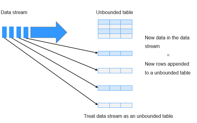
Figure 8 Unbounded table of Structured Streaming
Each query operation will generate a result table. At each trigger interval, updated data will be synchronized to the result table. Whenever the result table is updated, the updated result will be written into an external storage system.
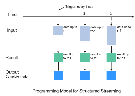
Figure 9 Structured Streaming data processing model
Storage modes of Structured Streaming at the output phase are as follows:
Complete Mode: The updated result sets are written into the external storage system. The write operation is performed by a connector of the external storage system.
Append Mode: If an interval is triggered, only added data in the result table will be written into an external system. This is applicable only on the queries where existing rows in the result table are not expected to change.
Update Mode: If an interval is triggered, only updated data in the result table will be written into an external system, which is the difference between the Complete Mode and Update Mode.
Basic Concepts
RDD
Resilient Distributed Dataset (RDD) is a core concept of Spark. It indicates a read-only and partitioned distributed dataset. Partial or all data of this dataset can be cached in the memory and reused between computations.
RDD Creation
An RDD can be created from the input of HDFS or other storage systems that are compatible with Hadoop.
A new RDD can be converted from a parent RDD.
An RDD can be converted from a collection of datasets through encoding.
RDD Storage
You can select different storage levels to store an RDD for reuse. (There are 11 storage levels to store an RDD.)
By default, the RDD is stored in the memory. When the memory is insufficient, the RDD overflows to the disk.
RDD Dependency
The RDD dependency includes the narrow dependency and wide dependency.
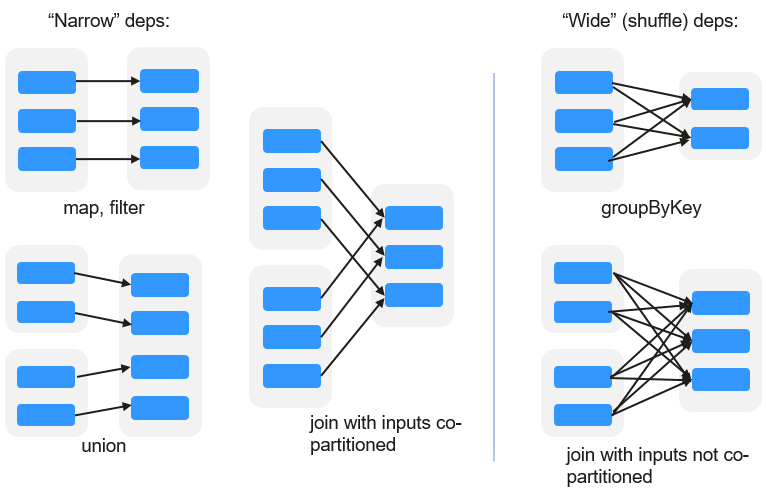
Figure 10 RDD dependency
Narrow dependency: Each partition of the parent RDD is used by at most one partition of the child RDD.
Wide dependency: Partitions of the child RDD depend on all partitions of the parent RDD.
The narrow dependency facilitates the optimization. Logically, each RDD operator is a fork/join (the join is not the join operator mentioned above but the barrier used to synchronize multiple concurrent tasks); fork the RDD to each partition, and then perform the computation. After the computation, join the results, and then perform the fork/join operation on the next RDD operator. It is uneconomical to directly translate the RDD into physical implementation. The first is that every RDD (even intermediate result) needs to be physicalized into memory or storage, which is time-consuming and occupies much space. The second is that as a global barrier, the join operation is very expensive and the entire join process will be slowed down by the slowest node. If the partitions of the child RDD narrowly depend on that of the parent RDD, the two fork/join processes can be combined to implement classic fusion optimization. If the relationship in the continuous operator sequence is narrow dependency, multiple fork/join processes can be combined to reduce a large number of global barriers and eliminate the physicalization of many RDD intermediate results, which greatly improves the performance. This is called pipeline optimization in Spark.
Transformation and Action (RDD Operations)
Operations on RDD include transformation (the return value is an RDD) and action (the return value is not an RDD). Figure 11 shows the RDD operation process. The transformation is lazy, which indicates that the transformation from one RDD to another RDD is not immediately executed. Spark only records the transformation but does not execute it immediately. The real computation is started only when the action is started. The action returns results or writes the RDD data into the storage system. The action is the driving force for Spark to start the computation.
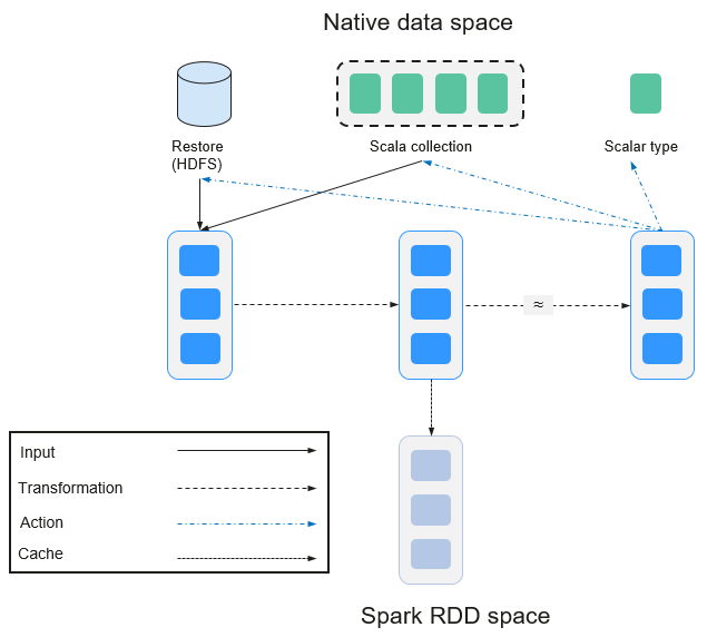
Figure 11 RDD operation
The data and operation model of RDD are quite different from those of Scala.
val file = sc.textFile("hdfs://...")
val errors = file.filter(_.contains("ERROR"))
errors.cache()
errors.count()
The textFile operator reads log files from the HDFS and returns files (as an RDD).
The filter operator filters rows with ERROR and assigns them to errors (a new RDD). The filter operator is a transformation.
The cache operator caches errors for future use.
The count operator returns the number of rows of errors. The count operator is an action.
Transformation includes the following types:
The RDD elements are regarded as simple elements.
The input and output has the one-to-one relationship, and the partition structure of the result RDD remains unchanged, for example, map.
The input and output has the one-to-many relationship, and the partition structure of the result RDD remains unchanged, for example, flatMap (one element becomes a sequence containing multiple elements after map and then flattens to multiple elements).
The input and output has the one-to-one relationship, but the partition structure of the result RDD changes, for example, union (two RDDs integrates to one RDD, and the number of partitions becomes the sum of the number of partitions of two RDDs) and coalesce (partitions are reduced).
Operators of some elements are selected from the input, such as filter, distinct (duplicate elements are deleted), subtract (elements only exist in this RDD are retained), and sample (samples are taken).
The RDD elements are regarded as key-value pairs.
Perform the one-to-one calculation on the single RDD, such as mapValues (the partition mode of the source RDD is retained, which is different from map).
Sort the single RDD, such as sort and partitionBy (partitioning with consistency, which is important to the local optimization).
Restructure and reduce the single RDD based on key, such as groupByKey and reduceByKey.
Join and restructure two RDDs based on the key, such as join and cogroup.
Note
The later three operations involving sorting are called shuffle operations.
Action includes the following types:
Generate scalar configuration items, such as count (the number of elements in the returned RDD), reduce, fold/aggregate (the number of scalar configuration items that are returned), and take (the number of elements before the return).
Generate the Scala collection, such as collect (import all elements in the RDD to the Scala collection) and lookup (look up all values corresponds to the key).
Write data to the storage, such as saveAsTextFile (which corresponds to the preceding textFile).
Check points, such as the checkpoint operator. When Lineage is quite long (which occurs frequently in graphics computation), it takes a long period of time to execute the whole sequence again when a fault occurs. In this case, checkpoint is used as the check point to write the current data to stable storage.
Shuffle
Shuffle is a specific phase in the MapReduce framework, which is located between the Map phase and the Reduce phase. If the output results of Map are to be used by Reduce, the output results must be hashed based on a key and distributed to each Reducer. This process is called Shuffle. Shuffle involves the read and write of the disk and the transmission of the network, so that the performance of Shuffle directly affects the operation efficiency of the entire program.
The figure below shows the entire process of the MapReduce algorithm.
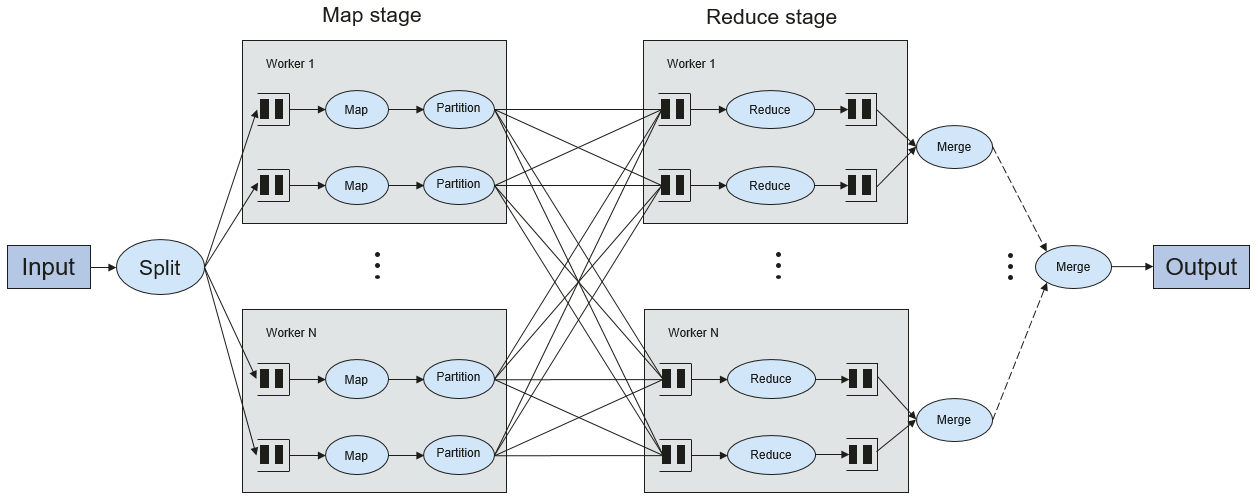
Figure 12 Algorithm process
Shuffle is a bridge to connect data. The following describes the implementation of shuffle in Spark.
Shuffle divides a job of Spark into multiple stages. The former stages contain one or more ShuffleMapTasks, and the last stage contains one or more ResultTasks.
Spark Application Structure
The Spark application structure includes the initialized SparkContext and the main program.
Initialized SparkContext: constructs the operating environment of the Spark Application.
Constructs the SparkContext object. The following is an example:
new SparkContext(master, appName, [SparkHome], [jars])
Parameter description:
master: indicates the link string. The link modes include local, Yarn-cluster, and Yarn-client.
appName: indicates the application name.
SparkHome: indicates the directory where Spark is installed in the cluster.
jars: indicates the code and dependency package of an application.
Main program: processes data.
For details about how to submit an application, visit https://spark.apache.org/docs/3.1.1/submitting-applications.html.
Spark Shell Commands
The basic Spark shell commands support the submission of Spark applications. The Spark shell commands are as follows:
./bin/spark-submit \
  --class <main-class> \
  --master <master-url> \
  ... # other options
  <application-jar> \
  [application-arguments]
Parameter description:
--class: indicates the name of the class of a Spark application.
--master: indicates the master to which the Spark application links, such as Yarn-client and Yarn-cluster.
application-jar: indicates the path of the JAR file of the Spark application.
application-arguments: indicates the parameter required to submit the Spark application. This parameter can be left blank.
Spark JobHistory Server
The Spark web UI is used to monitor the details in each phase of the Spark framework of a running or historical Spark job and provide the log display, which helps users to develop, configure, and optimize the job in more fine-grained units.